knitr::opts_chunk$set(warning=FALSE)
options(dplyr.summarise.inform = FALSE)
options(tigris_use_cache = TRUE)Spatial Accessibility
Background: What is r5r?
r5r is an R interface to the R5 routing engine, which allows for fast and efficient computation of public transit routes and accessibility to POIs quickly and efficiently based on travel times on a street network.
Using the package is straightforward but preparing the data for usage may not be. Here is how I have automated the process to get the the required (and optional) data into a directory that the package can utilize.
To demonstrate this, I will calculate accessibility to SAMSHA mental and behavioral health providers in the city of Cleveland.
setwd("C:/Users/barboza-salerno.1/Downloads/")
library(dplyr)
library(sf)
# remotes::install_github("ITSLeeds/osmextract")
library(osmextract)
library(raster)
library(stplanr)
library(tidytransit)
library(leaflet)
library(elevatr)
library(raster)
library(tidyverse)
library(hexbin)
library(tigris)
library(tidycensus)
library(purrr)
options(java.parameters = "-Xmx5G")
library(r5r)
library(akima)
library(gridExtra)
library(tmap)
library(tmaptools)
Requirements
This package requires the Java Development Kit version 11. OSU keeps overwriting it with each computer update. I have to re-install it by logging into this website and downloading this file. The requirement also makes the possibility of conflicts real. So, for example, if version 22 is installed along with 11 you may run into issues.
Comparison to Python and ArcGIS
There is a python module called r5py that provides similar functionality as r5r. It is probably even faster.
The main difference between ArcGIS besides the cost and interface is R’s flexibility, ease of data manipulation, and integration with other packages. UseR!
Overview of Required Data
- Street Network:
- .pbf format containing the street and pedestrian infrastructure;
- required;
- one file;
- street_network.osm.pbf
- Public transport network:
- GTFS data;
- can be more than 1 file;
- not required;
- public_transport_network.zip
- Topography:
- .tiff/.tif format;
- a raster containing the DEM;
- not required;
- one file;
- topography.tif
data_path <- "path/cleveland_access/accessdir"
fs::dir_tree(data_path)
path/cleveland_access/accessdir
├── cleveland_dem.tif
├── cleveland_gtfs.zip
├── hex_grid_data.csv
├── network.dat
├── network_settings.json
└── planet_-82.51,41.238_-80.958,41.61.osm.pbfDownloading and Cleaning the Street Network Data
There are several options for acquiring the street network data. However the data must be in protocol buffer format (pbf).
- Manually by going to the BBBike extract service

- Automatically using the
oemextractpackage: The osmextract package in R is a tool designed to facilitate the extraction and manipulation of OpenStreetMap (OSM) data, including information about roads, buildings, land use, and more.
The oe_providers() function helps users understand which data sources are available for extraction and what types of OSM data they provide.
print(oe_providers())Check the corresponding help pages to read more details about the fields in each database (e.g. ?geofabrik_zones) available_providers database_name number_of_zones number_of_fields
1 geofabrik geofabrik_zones 430 14
2 bbbike bbbike_zones 235 10
3 openstreetmap_fr openstreetmap_fr_zones 903 6#?geofabrik_zones
class(geofabrik_zones)[1] "sf" "data.frame"par(mar = rep(0.1, 4))
plot(geofabrik_zones[geofabrik_zones$level == 2, "name"], key.pos = NULL, main = NULL)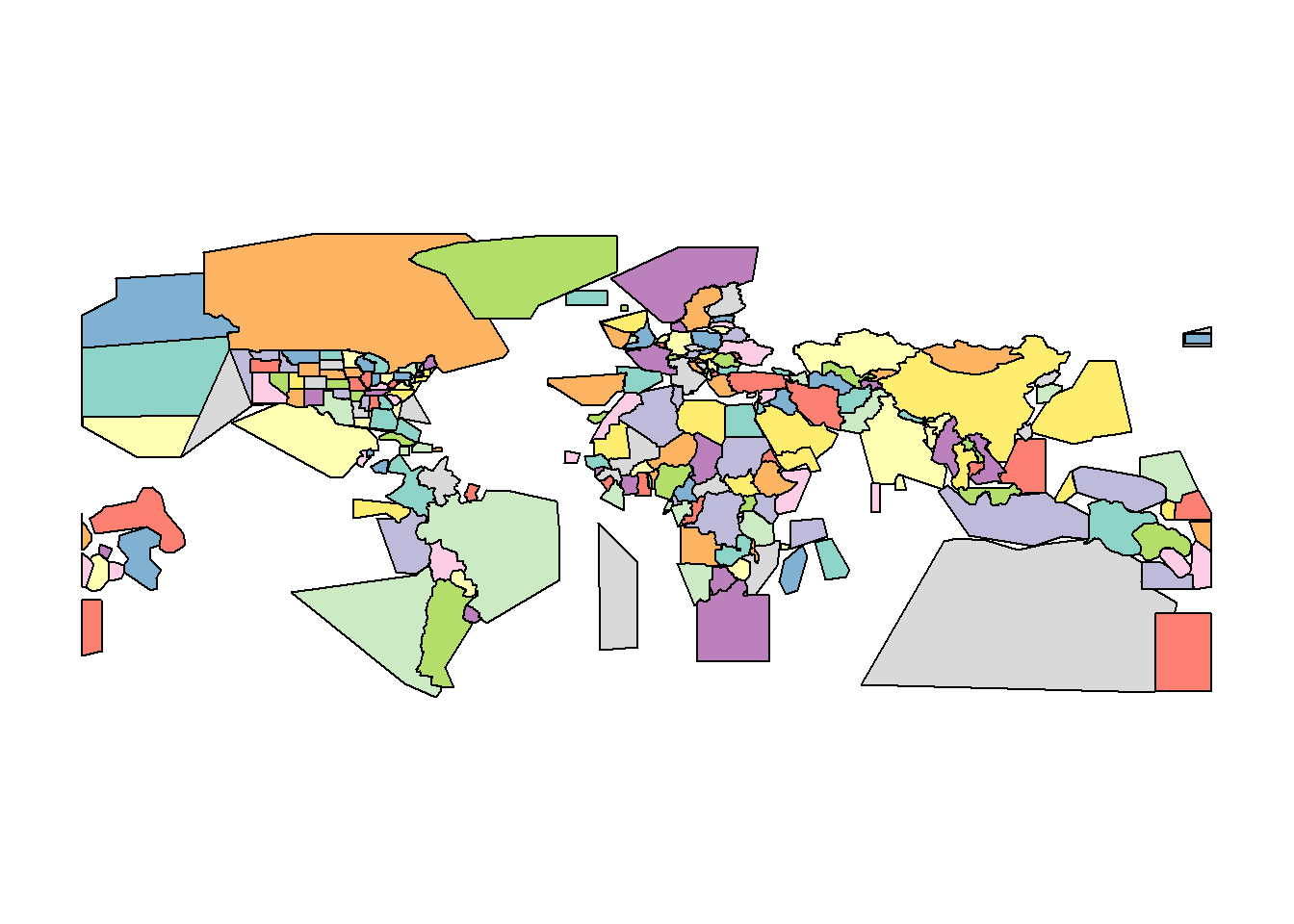
plot(bbbike_zones[bbbike_zones$level == 3, "name"], key.pos = NULL, main = NULL)
plot(openstreetmap_fr_zones[openstreetmap_fr_zones$level == 2, "name"], key.pos = NULL, main = NULL)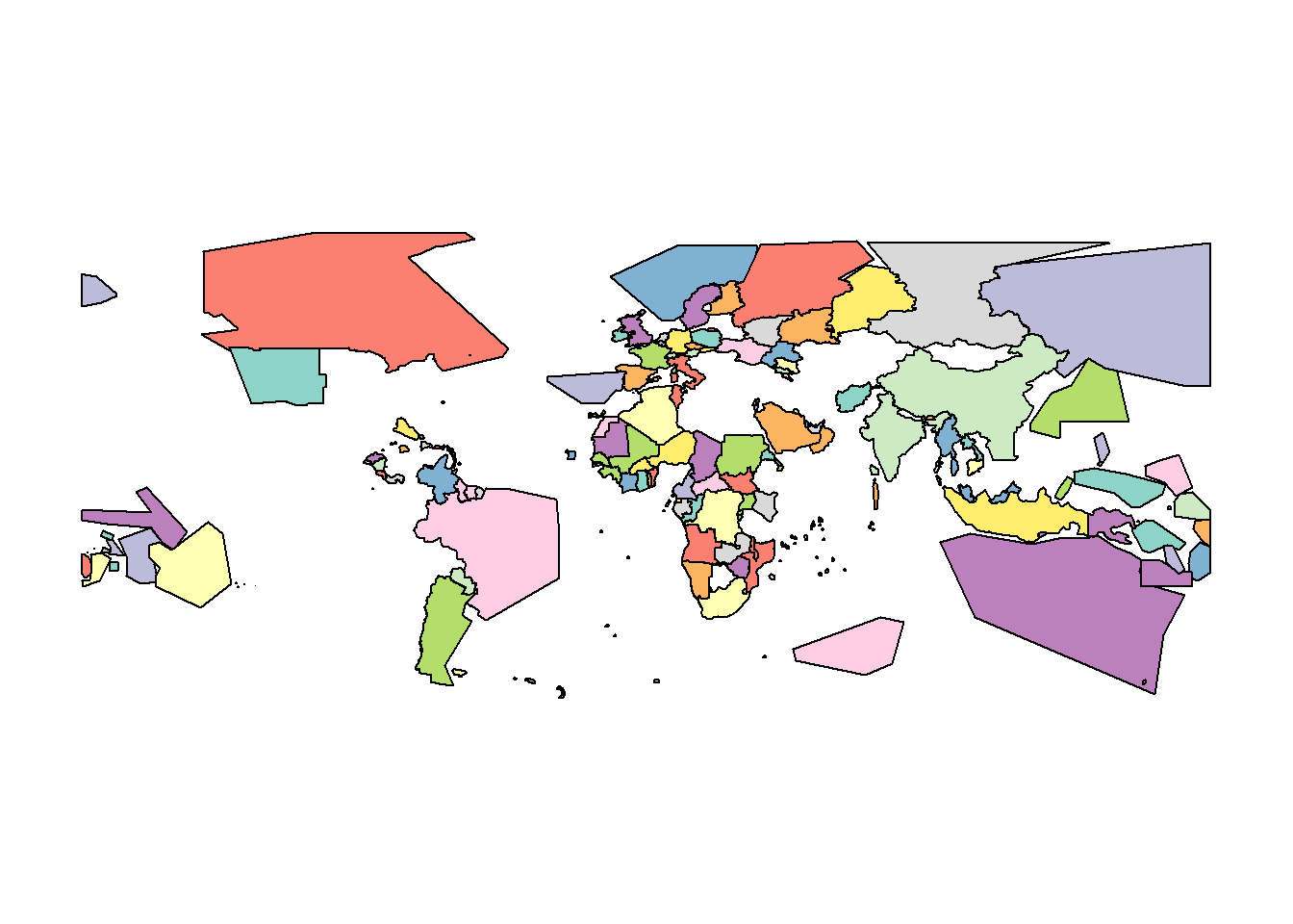
plot(openstreetmap_fr_zones[openstreetmap_fr_zones$level == 3, "name"], key.pos = NULL, main = NULL)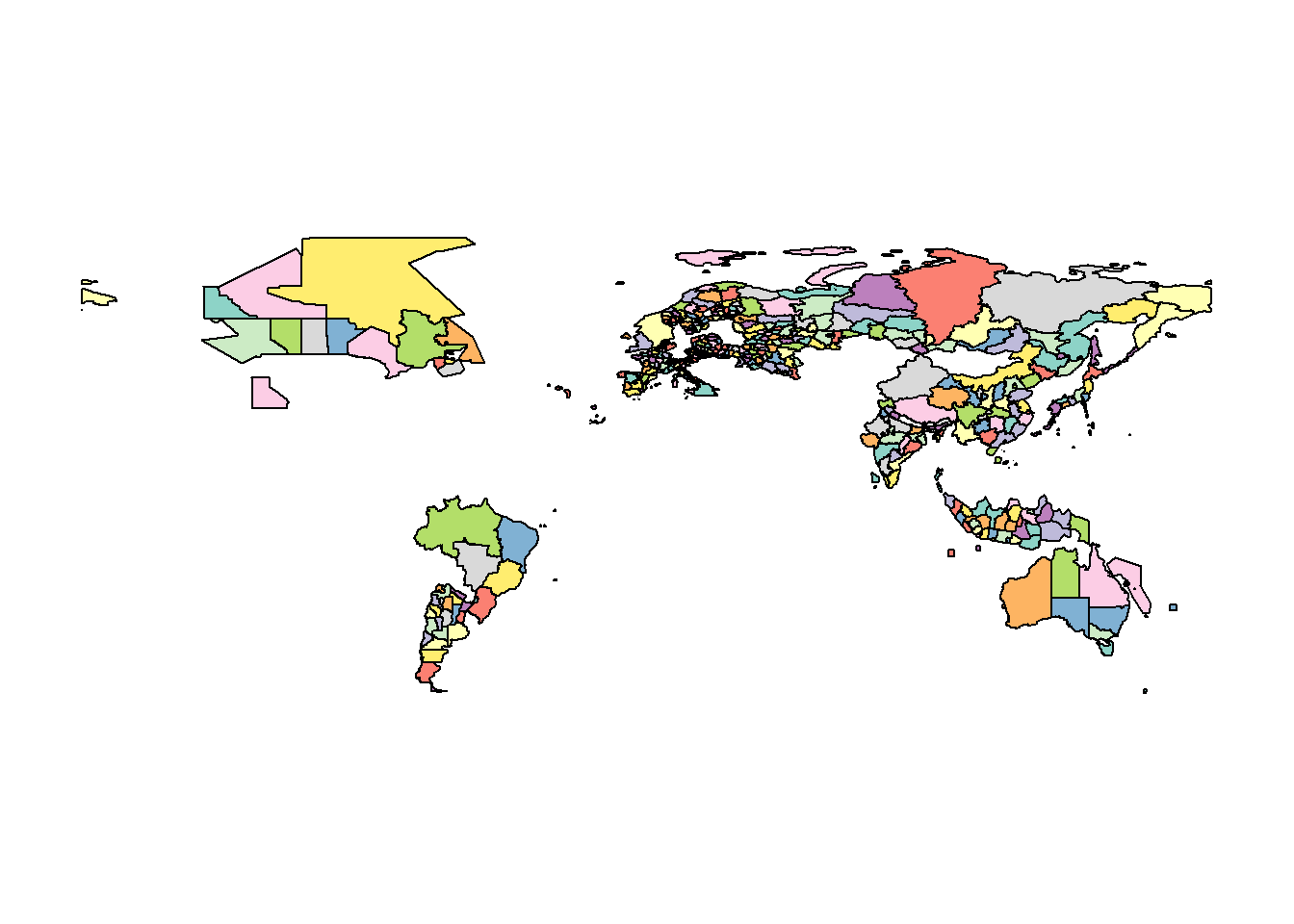
plot(openstreetmap_fr_zones[openstreetmap_fr_zones$level == 4, "name"], key.pos = NULL, main = NULL)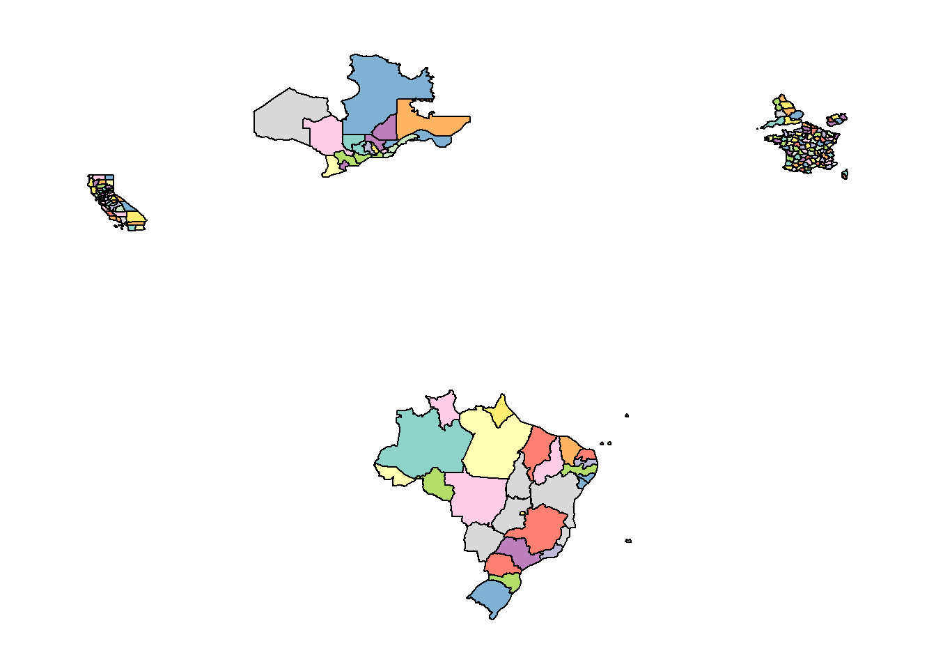
ohio_match <- oe_match("Ohio, USA", provider = "geofabrik")No exact match found for place = Ohio, USA and provider = geofabrik. Best match is China.
Checking the other providers.No exact match found in any OSM provider data. Searching for the location online.The input place was matched with us/ohio. oe_match_pattern("Ohio, USA")list()if (length(ohio_match) == 0) {
message("No datasets found for the specified location.")
} else {
print(ohio_match)
}$url
[1] "https://download.geofabrik.de/north-america/us/ohio-latest.osm.pbf"
$file_size
[1] 170527918oe_download_directory()[1] "C:\\Users\\barboza-salerno.1\\AppData\\Local\\Temp\\1\\RtmpAtp0Oq" oe_download(
file_url = ohio_match$url,
file_size = ohio_match$file_size,
provider = "geofabrik",
download_directory = "path"
)The chosen file was already detected in the download directory. Skip downloading.[1] "C:\\Users\\barboza-salerno.1\\Downloads\\path\\geofabrik_ohio-latest.osm.pbf"geofabrik_oh_gpkg = oe_vectortranslate("path/geofabrik_ohio-latest.osm.pbf")The corresponding gpkg file was already detected. Skip vectortranslate operations.Clipping the pbf file to your boundary file
Unless you are analyzing the state, the file will probably need to be clipped to the region you are analyzing, here the city of Cleveland.
First I will import the boundary file and get the bbox.
Second, I use a common tool to easily clip the pbf file from above to the city by entering the bbox coordinates into the program osmconvert below.
cleveland_bounds <- st_read("path/CLEV_bound.shp") %>% st_transform(crs=4326)Reading layer `CLEV_bound' from data source
`C:\Users\barboza-salerno.1\Downloads\path\CLEV_bound.shp'
using driver `ESRI Shapefile'
Simple feature collection with 1 feature and 17 fields
Geometry type: POLYGON
Dimension: XY
Bounding box: xmin: -9114737 ymin: 5070147 xmax: -9076206 ymax: 5101154
Projected CRS: WGS 84 / Pseudo-Mercatorst_bbox(cleveland_bounds) xmin ymin xmax ymax
-81.87908 41.39074 -81.53294 41.59937 plot(cleveland_bounds$geometry)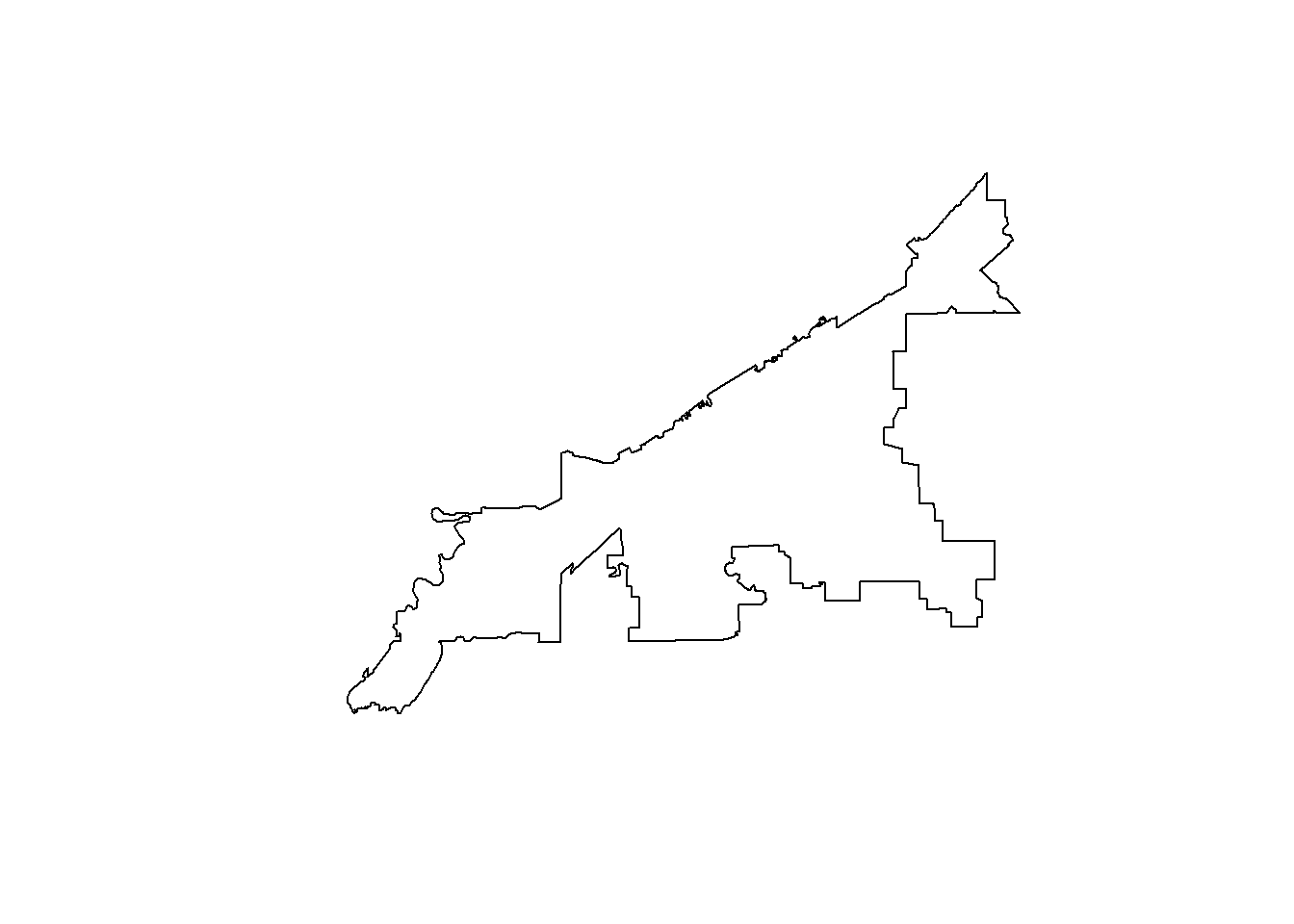
#st_write(cleveland_bounds, "path/cleveland_bounds.geojson")Clipping the pbf file to your location
To clip the file I use a command line tool called osmconvert. It has a nice wizard screen that moves you through the process.
As you can see below, I clipped the file using the bbox of the area associated with cleveland.
Osmconvert - OpenStreetMap Wiki

The size of the original file is about 242 MB but the clipped file is only about 8 MB

Get GTFS transit data
Next we need to identify and download the transit data. GTFS (General Transit Feed Specification) is a standard format for sharing public transportation schedules and associated data (e.g., stops, routes).
I googled it and found the files for Cleveland here.
In generaly, a good resource for transit data is OpenMobilityData TransitFeeds
gtfs_url <- "https://www.riderta.com/sites/default/files/gtfs/latest/google_transit.zip"

download.file(gtfs_url, destfile = file.path("path/cleveland_access", "cleveland_gtfs.zip"))

gtfs_data <- read_gtfs(file.path("path/cleveland_access", "cleveland_gtfs.zip"))head(gtfs_data$stops)# A tibble: 6 × 11
stop_id stop_code stop_name stop_desc stop_lat stop_lon zone_id stop_url
<chr> <chr> <chr> <chr> <dbl> <dbl> <chr> <chr>
1 00001 00001 COLUMBUS ST & … "" 41.4 -81.5 "" ""
2 00002 00002 10800 BROOKPAR… "" 41.4 -81.8 "" ""
3 00003 00003 BROADWAY & BOO… "" 41.5 -81.6 "" ""
4 00004 00004 EUCLID AV & E … "" 41.5 -81.6 "" ""
5 00005 00005 10081 W RIDGEW… "" 41.4 -81.8 "" ""
6 00006 00006 WASHINGTON AV … "" 41.5 -81.7 "" ""
# ℹ 3 more variables: location_type <int>, parent_station <chr>,
# wheelchair_boarding <int>head(gtfs_data$calendar)# A tibble: 6 × 10
service_id monday tuesday wednesday thursday friday saturday sunday start_date
<chr> <int> <int> <int> <int> <int> <int> <int> <date>
1 2408H-hh2… 1 1 1 1 1 0 0 2024-08-05
2 2408H-hh2… 0 0 0 0 0 1 0 2024-08-10
3 2408H-hh2… 0 0 0 0 0 0 1 2024-08-04
4 2408H-hh2… 0 0 0 0 0 0 1 2024-09-02
5 2408R-hr2… 1 1 1 1 1 0 0 2024-08-05
6 2408R-hr2… 1 1 1 1 1 0 0 2024-09-13
# ℹ 1 more variable: end_date <date>Visualize the stops
stops <- gtfs_data$stops

leaflet() %>%
  addTiles() %>%
  addCircleMarkers(data = stops, ~stop_lon, ~stop_lat,
                   popup = ~paste(stop_name, "<br>", stop_desc),
                   radius = .4,
                   color = "grey20",
                   fillOpacity = 0.7) %>%
  addPolygons(data = cleveland_bounds,
              color = "grey70",
              weight = 2,
              fillOpacity = 0.2)
Elevation Data (Optional)
This is optional but easy to get so I included it in the directory. To include elevation data, you have to first process the data and then compute elevation gradients.
The gradients then can be used to modify travel times to account for changes.
As an aside, the package called slopes is easy to use and can help visualize data from DEMs.
dem <- get_elev_raster(locations = cleveland_bounds, z = 10, clip = "locations")Mosaicing & ProjectingClipping DEM to locationsNote: Elevation units are in meters.plot(dem)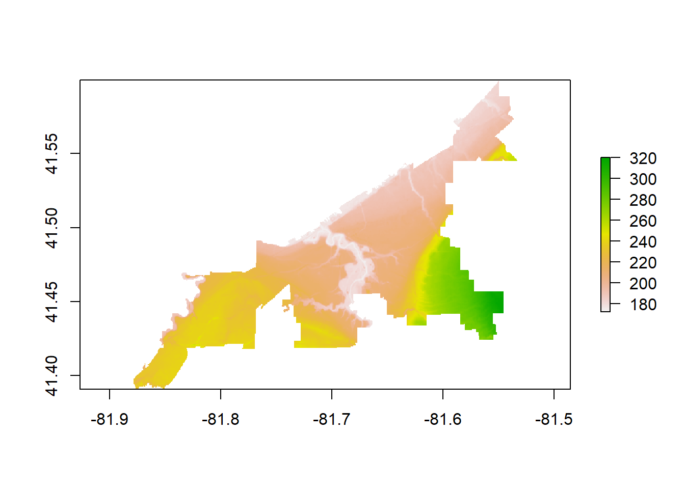
writeRaster(dem, filename = "path/cleveland_access/cleveland_dem.tif", format = "GTiff", overwrite = TRUE)Load the accessibility indicators
I clipped three data sets to the Cleveland boundary file:
abortion providers;
substance use facilities from the behavioral locator; and
opioid treatment facilities from the behavioral locator.
You can add all three indicators to the function at once by changing parameters of the opportunities_colname in the accessibility function below (e.g., from “su” to c(“su”, “otp”, etc)). Here I will focus on SU only.
#abortion_providers <- st_read("path/cleveland_access/abortion_providers.geojson") %>% st_transform(crs = 4326)
#otp_providers <- st_read("path/cleveland_access/otp_providers.geojson") %>% st_transform(crs = 4326)

su_providers <-
  st_as_sf(
    read.csv("path/cleveland_access/all_su_providers_in_county.csv"),
    coords = c("longitude", "latitude"),
    crs = 4326
    )
Next, the function requires a file that contains the geographic coordinates of the centroids of the polygons of an area, along with information about the number of amenities (as above). You can use census tracts or block groupsbut I decided to try hex grids.
sf_use_s2(FALSE)Spherical geometry (s2) switched offcleveland_bounds <- st_geometry(st_read("path/CLEV_bound.shp"))Reading layer `CLEV_bound' from data source
`C:\Users\barboza-salerno.1\Downloads\path\CLEV_bound.shp'
using driver `ESRI Shapefile'
Simple feature collection with 1 feature and 17 fields
Geometry type: POLYGON
Dimension: XY
Bounding box: xmin: -9114737 ymin: 5070147 xmax: -9076206 ymax: 5101154
Projected CRS: WGS 84 / Pseudo-Mercatorprojected_crs <- 5070
cleveland_bounds <- st_transform(cleveland_bounds, crs = projected_crs)
hex_grid <- st_make_grid(
cleveland_bounds,
cellsize = 500,
square = FALSE
) %>%
st_as_sf() %>%
tigris::erase_water() %>%
st_intersection(cleveland_bounds) %>%
st_transform(crs = projected_crs) %>%
mutate(id = row_number()) Fetching area water data for your dataset's location...Erasing water area...
If this is slow, try a larger area threshold value.hex_grid <- hex_grid %>%
filter(st_geometry_type(.) %in% c("POLYGON", "MULTIPOLYGON"))Intersect the hex grid and CBG data by area
I want to get the counts in hex grids before doing the analysis.
intersections <- st_intersection(hex_grid, acs_data) %>%
  mutate(area_intersection = st_area(.))

intersections <-
  intersections %>%
  mutate(
    proportion = as.numeric(area_intersection / area_cbg),
    num_black = proportion * B03002_003E,
    total_population = proportion * B01001_001E,
    num_women = proportion * B01001_026E
    )

hex_grid_aggregated <-
  intersections %>%
  st_drop_geometry() %>%
  group_by(id) %>%
  summarize(num_black = sum(num_black, na.rm = TRUE),
    total_population = sum(total_population, na.rm = TRUE),
    num_women = sum(num_women, na.rm = TRUE)
    )

hex_grid <- hex_grid %>%
  left_join(
    hex_grid_aggregated, by = "id"
    ) %>%
  replace_na(
    list(num_black = 0, total_population = 0, num_women = 0)
    )  # No intersecting CBGs

hex_grid <- st_transform(hex_grid, crs = 4326)

hex_grid <- hex_grid %>%
  mutate(num_black = round(num_black, 0),
     black_percentage = ifelse(total_population > 0, (num_black / total_population) * 100, 0),
     num_women = round(num_women, 0),
     women_percentage = ifelse(total_population > 0, (num_women / total_population) * 100, 0)
     )

total_black_cbg <- sum(acs_data$B03002_003E, na.rm = TRUE)
total_black_hex <- sum(hex_grid$num_black, na.rm = TRUE)
total_women_cbg <- sum(acs_data$B01001_026E, na.rm = TRUE)
total_women_hex <- sum(hex_grid$num_women, na.rm = TRUE)print(paste("Total Black individuals in CBGs:", total_black_cbg))[1] "Total Black individuals in CBGs: 163485"print(paste("Total Black individuals in Hex Grid:", total_black_hex))[1] "Total Black individuals in Hex Grid: 162651"print(paste("Total women in CBGs:", total_women_cbg))[1] "Total women in CBGs: 236434"print(paste("Total women in Hex Grid:", total_women_hex))[1] "Total women in Hex Grid: 235863"Get Hex Grid centroids which servce as O-D
hex_centroids <- st_centroid(hex_grid)Aggregate SU Providers to Hex Grids
#hex_grid$abortion <- lengths(st_intersects(hex_grid, abortion_providers))
#hex_grid$otp <- lengths(st_intersects(hex_grid, otp_providers))
hex_grid$su <- lengths(st_intersects(hex_grid, su_providers))
although coordinates are longitude/latitude, st_intersects assumes that they
are planarFormatting the POI data
Note, the r5r package requires the POI data to have a specific format that includes columns called id, lat and lon
hex_data <- cbind(hex_grid, st_coordinates(hex_centroids)) %>%
  dplyr::rename(lon = X, lat = Y)

head(hex_data)
Simple feature collection with 6 features and 9 fields
Geometry type: POLYGON
Dimension: XY
Bounding box: xmin: -81.87908 ymin: 41.39074 xmax: -81.86818 ymax: 41.40768
Geodetic CRS: WGS 84
id num_black total_population num_women black_percentage women_percentage su
1 1 94 166.2951 87 56.52602 52.31664 0
2 2 113 199.9269 105 56.52065 52.51919 0
3 3 132 235.0009 123 56.17000 52.34023 0
4 4 223 395.4318 207 56.39405 52.34784 0
5 5 0 0.0000 0 0.00000 0.00000 0
6 6 0 0.0000 0 0.00000 0.00000 0
lon lat x
1 -81.87711 41.39833 POLYGON ((-81.87539 41.3998...
2 -81.87607 41.39487 POLYGON ((-81.8759 41.39729...
3 -81.87367 41.40127 POLYGON ((-81.87215 41.4007...
4 -81.87519 41.39207 POLYGON ((-81.8737 41.39313...
5 -81.87266 41.39823 POLYGON ((-81.87539 41.3998...
6 -81.86965 41.40554 POLYGON ((-81.86879 41.4073...write.csv(st_drop_geometry(hex_data), "path/cleveland_access/accessdir/hex_grid_data.csv", row.names = FALSE)ggplot() +
geom_sf(data = hex_grid, aes(fill = num_women), color = NA) +
scale_fill_viridis_c(name = "Number of Women") +
labs(title = "Number of Women in Each Hex Grid Cell") +
theme_void()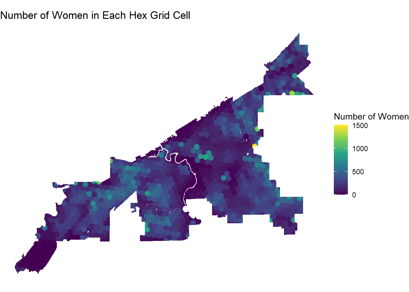
ggplot() +
  geom_sf(data = hex_grid, aes(fill = black_percentage), color = NA) +
  scale_fill_viridis_c(name = "% Black") +
  labs(title = "Percent Black in Each Hex Grid Cell") +
  theme_void()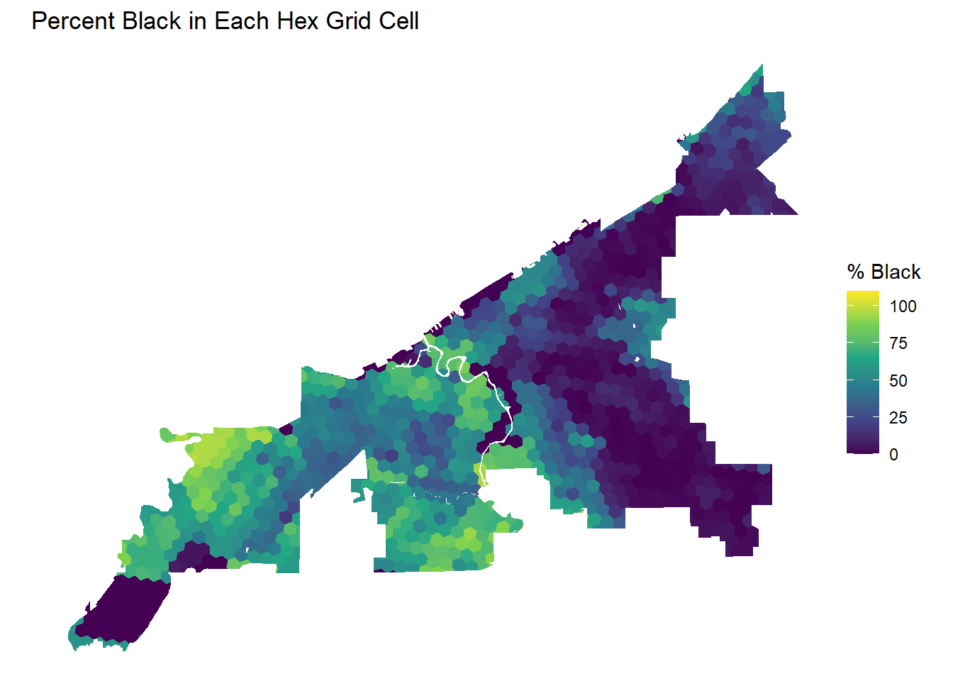
ggplot() +
  geom_sf(data = hex_grid, aes(fill = su), color = NA) +
  scale_fill_viridis_c(name = "Number of SUPs") +
  labs(title = "Number of SUPs in Each Hex Grid Cell") +
  theme_void()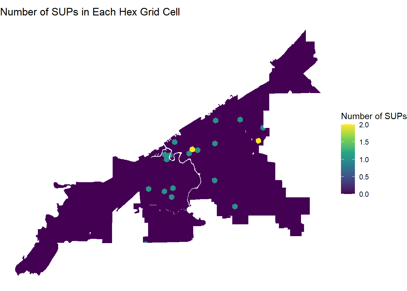
data_path <- "path/cleveland_access/accessdir"
fs::dir_tree(data_path)
path/cleveland_access/accessdir
├── cleveland_dem.tif
├── cleveland_gtfs.zip
├── hex_grid_data.csv
├── network.dat
├── network_settings.json
└── planet_-82.51,41.238_-80.958,41.61.osm.pbfr5r_core <- setup_r5(data_path, verbose = FALSE)Using cached R5 version from C:/Users/barboza-salerno.1/AppData/Local/R/win-library/4.2/r5r/jar/r5-v6.9-all.jar
Using cached network.dat from path/cleveland_access/accessdir/network.dat# read data.frame with grid centroids
points <- data.table::fread(file.path(data_path, "hex_grid_data.csv"), colClasses = c("id" = "character"))
ttm <- travel_time_matrix(
r5r_core,
origins = points,
destinations = points,
mode = c("WALK", "TRANSIT"),
departure_datetime = as.POSIXct(
"13-05-2024 14:00:00", #note change as necessary
format = "%d-%m-%Y %H:%M:%S"
),
max_walk_time = 30,
max_trip_duration = 120,
verbose = FALSE,
progress = FALSE
)
head(ttm) from_id to_id travel_time_p50
<char> <char> <int>
1: 1 1 1
2: 1 3 11
3: 1 5 13
4: 1 6 21
5: 1 8 23
6: 1 9 27The Accessibility Function
Finally, we can use the r5r package to calculate accessibility measures based on the network and transit system.
Both origins and destinations are specified as points, based on the centroids of the CBGs above.
The opportunities column contains the opportunities attributes. The decay funciton is using a step function where the accessibility value is constant within a given range and drops to zero beyond that range.
Cutoff determines the cutoff time for the decay function. Here we use 30 minutes by transit and walking, meaning that accessibility values will only consider trips that are 30 min. or less.
The mode indicates we want to consider transit + walk times.
The departure date provides the date of departure, which may significantly alter the analysis. The maximum total duration (in minutes) for trips, including both walking and transit times. Here it is set to 120 minutes.
r5r_access_Monday_2PM <- accessibility(
  r5r_core,
  origins = points,
  destinations = points,
  opportunities_colname = "su",
  decay_function = "step",
  cutoffs = 30,
  mode = c("WALK", "TRANSIT"),
  departure_datetime = as.POSIXct(
    "13-05-2024 14:00:00", # Monday May 13, 2024.
    format = "%d-%m-%Y %H:%M:%S"
  ),
  max_walk_time = 30,
  max_trip_duration = 120,
  verbose = FALSE,
  progress = FALSE
)

head(r5r_access_Monday_2PM)
id opportunity percentile cutoff accessibility
<char> <char> <int> <int> <num>
1: 1 su 50 30 0
2: 2 su 50 30 0
3: 3 su 50 30 0
4: 4 su 50 30 0
5: 5 su 50 30 0
6: 6 su 50 30 0access.interp <- r5r_access_Monday_2PM %>%
inner_join(points, by=c('id'='id')) %>%
with(interp(lon, lat, accessibility)) %>%
with(cbind(acc=as.vector(z), # Column-major order
x=rep(x, times=length(y)),
y=rep(y, each=length(x)))) %>%
as.data.frame() %>%
na.omit()
bb_x <- c(min(access.interp$x), max(access.interp$x))
bb_y <- c(min(access.interp$y), max(access.interp$y))
# extract OSM network, to plot over map, I only did this for the last map since it takes time
street_net <- street_network_to_sf(r5r_core)# plot
ggplot(na.omit(access.interp)) +
geom_contour_filled(aes(x=x, y=y, z=acc), alpha=.8) +
# geom_sf(data = street_net$edges, color = "gray55", size=0.07, alpha = 0.3) +
scale_fill_viridis_d(direction = -1, option = 'B') +
scale_x_continuous(expand=c(0,0)) +
scale_y_continuous(expand=c(0,0)) +
coord_sf(xlim = bb_x, ylim = bb_y) +
labs(fill = "Substance Use Facilities\n30 minutes\n(median travel time)") +
theme_void() +
theme(axis.title = element_blank())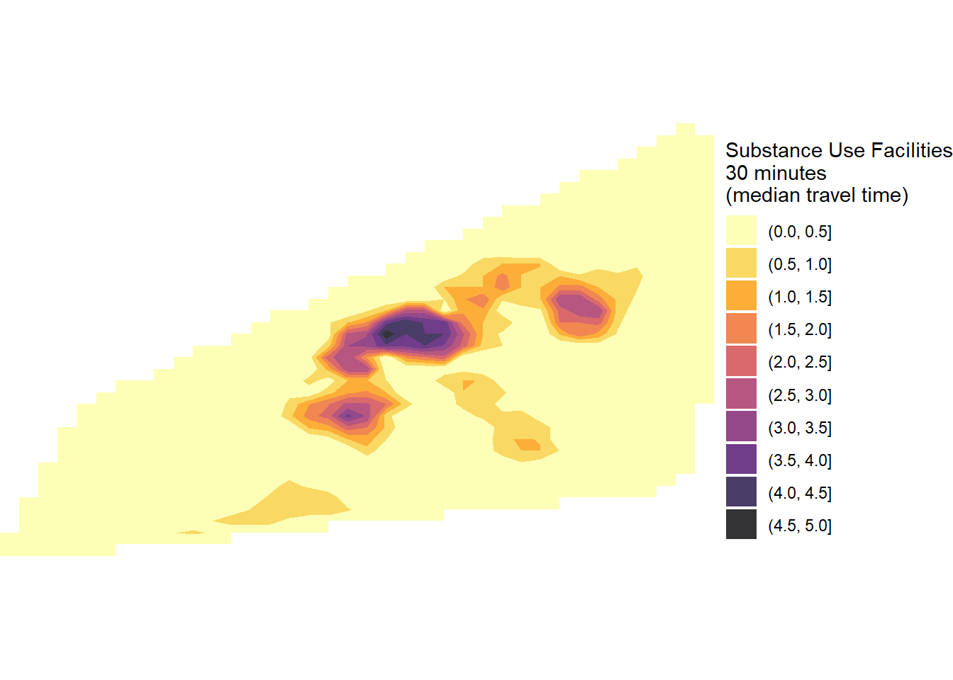
r5r_access_Sunday_7PM <- accessibility(
  r5r_core,
  origins = points,
  destinations = points,
  opportunities_colname = "su",
  decay_function = "step",
  cutoffs = 30,
  mode = c("WALK", "TRANSIT"),
  departure_datetime = as.POSIXct(
    "12-05-2024 19:00:00", #Sunday May 12, 2024.
    format = "%d-%m-%Y %H:%M:%S"
  ),
  max_walk_time = 15,
  max_trip_duration = 60,
  verbose = FALSE,
  progress = FALSE
)

head(r5r_access_Sunday_7PM)
id opportunity percentile cutoff accessibility
<char> <char> <int> <int> <num>
1: 1 su 50 30 0
2: 2 su 50 30 0
3: 3 su 50 30 0
4: 4 su 50 30 0
5: 5 su 50 30 0
6: 6 su 50 30 0access.interp <- r5r_access_Sunday_7PM %>%
inner_join(points, by=c('id'='id')) %>%
with(interp(lon, lat, accessibility)) %>%
with(cbind(acc=as.vector(z), # Column-major order
x=rep(x, times=length(y)),
y=rep(y, each=length(x)))) %>%
as.data.frame() %>%
na.omit()
# find results' bounding box to crop the map
bb_x <- c(min(access.interp$x), max(access.interp$x))
bb_y <- c(min(access.interp$y), max(access.interp$y))ggplot(na.omit(access.interp)) +
geom_contour_filled(aes(x=x, y=y, z=acc), alpha=.8) +
# geom_sf(data = street_net$edges, color = "gray55", size=0.07, alpha = 0.3) +
scale_fill_viridis_d(direction = -1, option = 'B') +
scale_x_continuous(expand=c(0,0)) +
scale_y_continuous(expand=c(0,0)) +
coord_sf(xlim = bb_x, ylim = bb_y) +
labs(fill = "Substance Use Facilities\n15 minutes\n(median travel time)") +
theme_void() +
theme(axis.title = element_blank())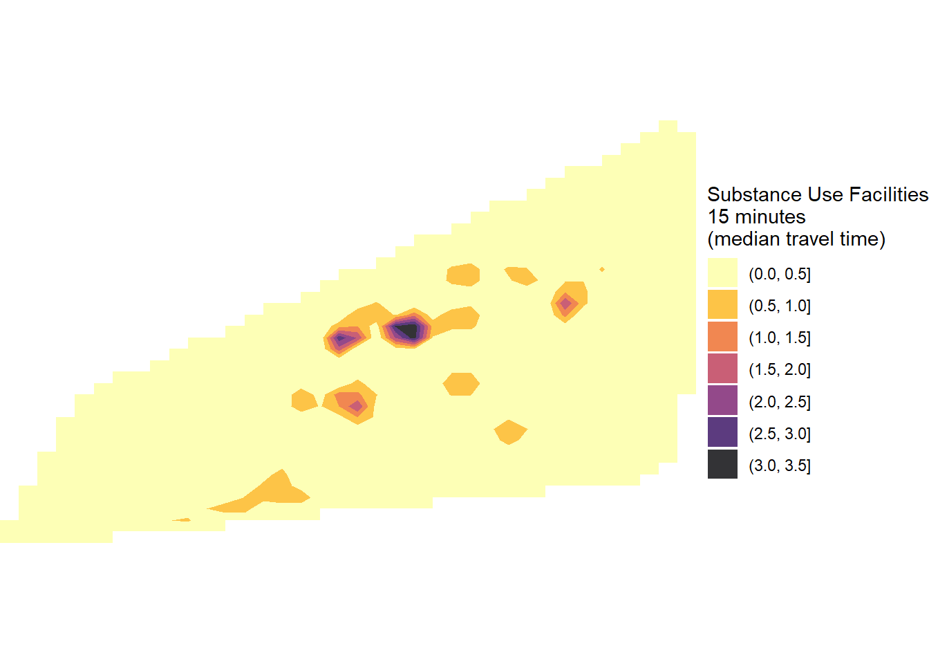
r5r_access_CAR_5min <- accessibility(
  r5r_core,
  origins = points,
  destinations = points,
  opportunities_colname = "su",
  decay_function = "step",
  cutoffs = 5,
  mode = c("CAR"),
  max_trip_duration = 20,
  verbose = FALSE,
  progress = FALSE
)

head(r5r_access_CAR_5min)
id opportunity percentile cutoff accessibility
<char> <char> <int> <int> <num>
1: 1 su 50 5 0
2: 2 su 50 5 0
3: 3 su 50 5 0
4: 4 su 50 5 0
5: 5 su 50 5 0
6: 6 su 50 5 0access.interp <- r5r_access_CAR_5min %>%
inner_join(points, by=c('id'='id')) %>%
with(interp(lon, lat, accessibility)) %>%
with(cbind(acc=as.vector(z), # Column-major order
x=rep(x, times=length(y)),
y=rep(y, each=length(x)))) %>%
as.data.frame() %>%
na.omit()
bb_x <- c(min(access.interp$x), max(access.interp$x))
bb_y <- c(min(access.interp$y), max(access.interp$y))Visualizing
I tried to make the plot prettier by clipping the results to the boundary
cleveland_bounds <- cleveland_bounds %>%
  st_transform(crs(street_net$edges))
access_sf <- st_as_sf(access.interp, coords = c("x", "y"), crs = 4326) # Replace 4326 with your CRS if different
access_clipped <- st_intersection(access_sf, cleveland_bounds)
although coordinates are longitude/latitude, st_intersection assumes that they
are planarstreet_edges_sf <- st_as_sf(street_net$edges)
street_edges_clipped <- st_intersection(street_edges_sf, cleveland_bounds)although coordinates are longitude/latitude, st_intersection assumes that they
are planarggplot() +
geom_contour_filled(data = na.omit(access_clipped),
aes(x = st_coordinates(access_clipped)[,1],
y = st_coordinates(access_clipped)[,2], z = acc), alpha = .8) +
geom_sf(data = street_edges_clipped, color = "gray75", size = 0.06, alpha = 0.25) +
geom_sf(data = cleveland_bounds, fill = NA, color = "black", size = 0.5) + # Add city boundary
scale_fill_viridis_d(direction = -1, option = 'B') +
scale_x_continuous(expand = c(0, 0)) +
scale_y_continuous(expand = c(0, 0)) +
coord_sf() +
labs(fill = "Substance Use Facilities\n5 minutes DRIVE \n(median travel time)") +
theme_void() +
theme(axis.title = element_blank())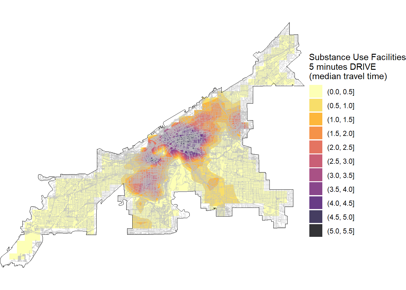
Caclulate Disparities in Accessibility for r5r_access_Sunday_7PM
hex_grid$id <- as.character(as.numeric(hex_grid$id))
hex_grid <- r5r_access_Monday_2PM %>%
  dplyr::select(id, accessibility) %>%
  left_join(hex_grid)
Joining with `by = join_by(id)`hex_grid <- hex_grid %>% st_as_sf() %>%
mutate(black_percentage_quartile = ntile(black_percentage, 4)) %>% na.omit()
quartile_summary <- hex_grid %>%
group_by(black_percentage_quartile) %>%
summarize(mean_accessibility = mean(accessibility, na.rm = TRUE),
median_accessibility = median(accessibility, na.rm = TRUE),
.groups = 'drop')although coordinates are longitude/latitude, st_union assumes that they are
planarprint(quartile_summary)Simple feature collection with 4 features and 3 fields
Geometry type: MULTIPOLYGON
Dimension: XY
Bounding box: xmin: -81.87908 ymin: 41.39074 xmax: -81.53294 ymax: 41.59928
Geodetic CRS: WGS 84
# A tibble: 4 × 4
black_percentage_quartile mean_accessibility median_accessibility
<int> <dbl> <dbl>
1 1 0.167 0
2 2 0.572 0
3 3 0.691 0
4 4 0.255 0
# ℹ 1 more variable: x <MULTIPOLYGON [°]>plot_black_percentage <- ggplot(hex_grid) +
geom_sf(aes(fill = black_percentage)) +
scale_fill_viridis_c(option = "plasma", name = "Black Percentage") +
theme_void() +
labs(title = "Map of Black Percentage Across Hex Grid",
caption = "Source: American Community Survey (2020)")
plot_accessibility <- ggplot(hex_grid) +
geom_sf(aes(fill = accessibility)) +
scale_fill_viridis_c(option = "plasma", name = "Accessibility") +
theme_void() +
labs(title = "Map of Accessibility Across Hex Grid",
caption = "Source: SAMSHA Behavioral Health Locator")
grid.arrange(plot_black_percentage, plot_accessibility, ncol = 1)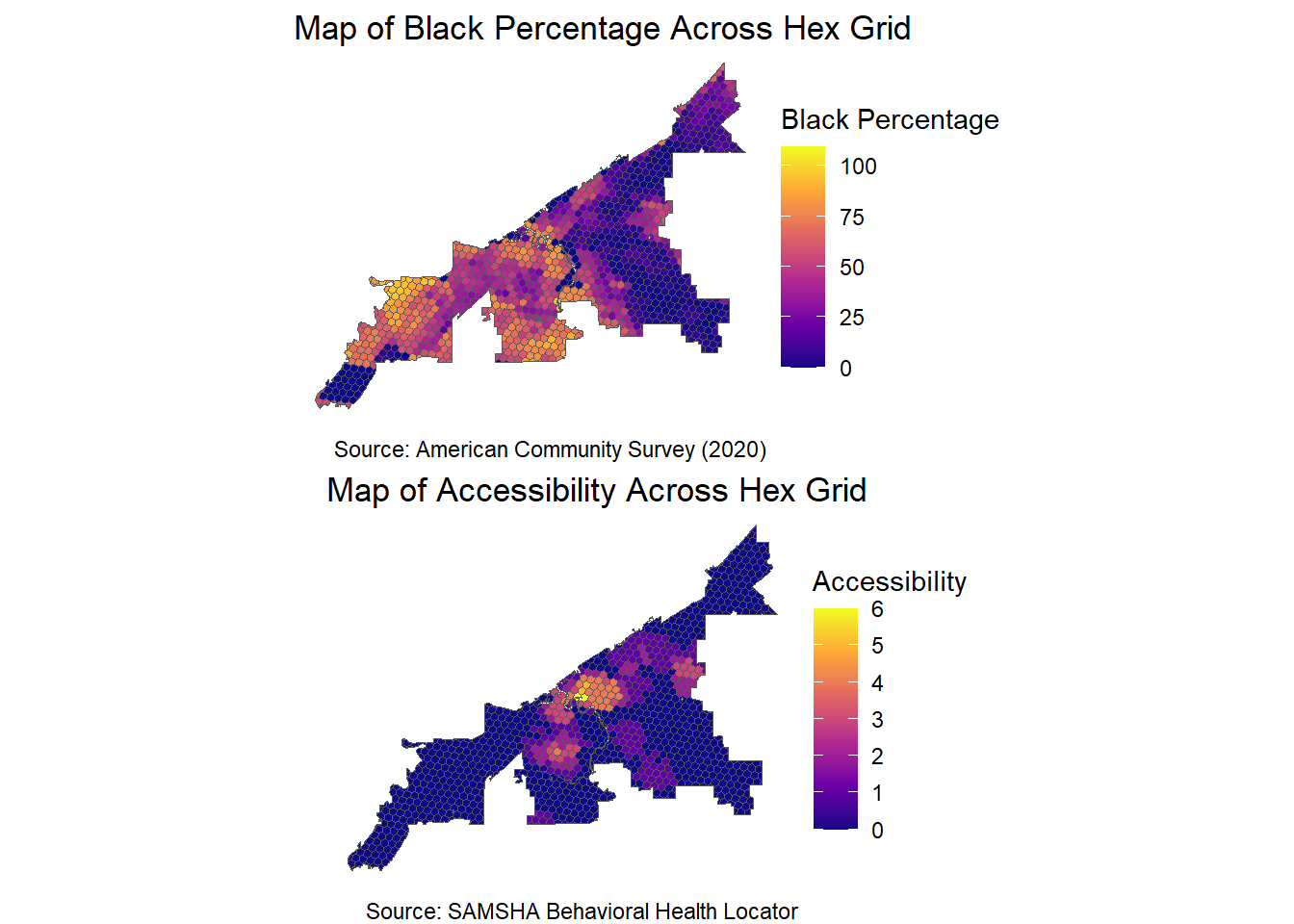
breaks = c(0, 1, 2, 3, 4, 5, 6)
cleveland_bounds <- cleveland_bounds %>% st_transform(4326)

shapes <- gtfs_data$shapes

shapes_list <- split(shapes, shapes$shape_id)
line_features <- lapply(shapes_list, function(df) {
  st_linestring(as.matrix(df[, c("shape_pt_lon", "shape_pt_lat")]))
})

shapes_sf <- st_sfc(line_features, crs = 4326)
shapes_sf <- st_sf(shape_id = names(shapes_list), geometry = shapes_sf)
clipped_lines_sf <- st_intersection(shapes_sf, cleveland_bounds)
although coordinates are longitude/latitude, st_intersection assumes that they
are planarbreaks = c(0, 1, 2, 3, 4, 5, 6)
tm_shape(hex_grid) +
tm_fill("accessibility",
breaks = breaks,
palette = 'GnBu',
#legend.hist = TRUE,
title = "SU Providers \n(15 min Travel, Public Transit, \n7:00 PM Sunday)") +
tm_layout(title = "Cleveland, Ohio",
title.size = 1.5,
title.color = "azure4",
title.position = c("left", "top"),
inner.margins = c(0.09, 0.10, 0.10, 0.08),
fontfamily = 'Georgia',
#bg.color = "grey95",
frame = TRUE) +
tm_borders(col = "grey40", lwd = 0.1)+
tm_legend(title.size=0.9,
text.size = 0.6,
#frame = "grey",
position = c("left", "top")) +
tm_scale_bar(color.dark = "gray60",
position = c("left", "bottom")) +
tm_shape(clipped_lines_sf) +
tm_lines(col = 'indianred', lwd = 1, alpha = 0.4) +
tm_add_legend(type = "line", labels = 'Cleveland Regional Transit Authority', col = 'indianred' ) 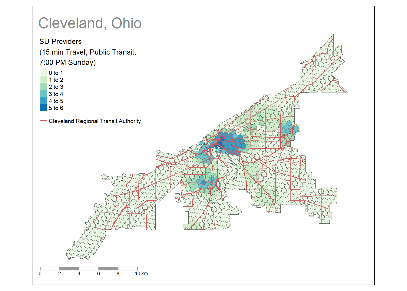
Clean up
rm(r5r_core)
gc()
used (Mb) gc trigger (Mb) max used (Mb)
Ncells 6895236 368.3 12955847 692.0 12955847 692.0
Vcells 28490302 217.4 55485308 423.4 55485302 423.4
Social Vulnerability Analysis
The end goal is to examine how accessibility changes according to population characteristics.
I am studying abortion so I downloaded the count of the female population in CBGs from the ACS.
I also get counts for the population of Black individuals in each CBG, and then calculate the percentage of each.
My key is installed.
You can modify this to include rural-urban classification data. You don’t have to do the hex grids, but it is a common way to visualize accessibility.