How to Analyze Caselaw Using CourtListener's API in R
A Tutorial for the Analysis of Legal Text
I previously showed how to pull ‘Indian’ Child Welfare Act (ICWA) cases using the Caselaw Access Project (Harvard Law). That API has since changed. This post updates the workflow using the Free Law Project’s CourtListener, which now partners with Harvard to make this data freely available.
Finding the Cases
Start at the CourtListener website and search for “Indian Child Welfare Act” (or “icwa”).

You’ll see a page of opinion results.
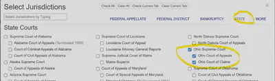
Filtering by Jurisdiction
Click Select Jurisdiction → State. Clear all, then select:
- Ohio Supreme Court
- Ohio Court of Appeals
- Ohio Court of Claims
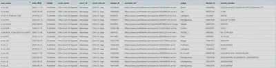
This gives you a quick check on the expected volume so you can validate the code’s output below.
The site reported 36 cases from Ohio when this tutorial was written. Note that the exact number may change over time as new opinions are added or metadata is corrected.
Getting the Data into R
The Search API returns clean JSON results by querying for opinions that contain the exact phrase “indian child welfare act”, restricting to published opinions, ordering by relevance, and (optionally) limiting the results to three Ohio courts.
Required Libraries
library(httr2)
library(purrr)
library(dplyr)
library(tibble)
library(tidyr)
library(stringr)
API Configuration
SEARCH_BASE <- "https://www.courtlistener.com/api/rest/v4/search/"
UA <- "R/httr2 (your-email-address) – ICWA metadata collection"

query_params <- list(
  q = '"indian child welfare act"',
  type = "o",
  order_by = "score desc",
  stat_Published = "on",
  court = "ohio ohioctapp ohioctcl" # optional: specify the court name
)
Helper Functions
pull_chr <- function(x, ...) {
  v <- purrr::pluck(x, ..., .default = NA)
  if (is.null(v) || length(v) == 0) return(NA_character_)
  as.character(v)
}

pull_num <- function(x, ...) {
  v <- purrr::pluck(x, ..., .default = NA_real_)
  suppressWarnings(as.numeric(v))
}

get_json <- function(url) {
  resp <- request(url) |>
    req_user_agent(UA) |>
    req_url_query() |>
    req_perform()
  resp_check_status(resp)
  resp_body_json(resp, simplifyVector = FALSE)
}
Fetching Search Results
fetch_search_pages <- function() {
  req <- request(SEARCH_BASE) |>
    req_user_agent(UA) |>
    req_url_query(!!!query_params)

  dat <- req |>
    req_perform() |>
    (\(r){
      resp_check_status(r)
      resp_body_json(r, simplifyVector=FALSE)
    })()

  pages <- list(dat)

  while (!is.null(dat$`next`)) {
    dat <- request(dat$`next`) |>
      req_user_agent(UA) |>
      req_perform() |>
      (\(r){
        resp_check_status(r)
        resp_body_json(r, simplifyVector=FALSE)
      })()
    pages <- append(pages, list(dat))
  }

  pages
}

pages   <- fetch_search_pages()
results <- pages |> map("results") |> flatten()
results is a list of per-case records from the API. Each element includes:
- Case name
- Filing date
- Court identifiers
- Citation strings
- Public URL where the caselaw text is available
- Other relevant metadata
Creating a Dataframe
For Ohio, this produced ~35 unique case names versus 36 displayed on the site. In comparing the case_name variable to the search results, you can reconcile the discrepancy.

Minor discrepancies happen because search hits can include multiple opinions or siblings per matter, and because the index is updated over time.
Downloading Case Text
Each opinion has an API endpoint with plain text and HTML fields. A small function can loop over the URL field, request the text, and save one .txt file per opinion. A short pause between requests is included and retried if necessary.
# Example function to download case text
download_case_text <- function(case_url, output_dir) {
  # Add rate limiting
  Sys.sleep(1)

  # Request the case data
  case_data <- get_json(case_url)

  # Extract plain text
  case_text <- pull_chr(case_data, "plain_text")

  # Save to file
  file_name <- paste0(output_dir, "/",
                     gsub("[^A-Za-z0-9]", "_", pull_chr(case_data, "case_name")),
                     ".txt")
  writeLines(case_text, file_name)
}
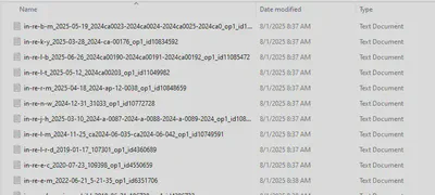
Remember to be considerate of rate limits and to include a User Agent string with your contact information.
Visualizing the Results
You can use ggplot2 to visualize the results, for example:
Filings by Year
library(ggplot2)

# Assuming you have a dataframe with filing dates
cases_df %>%
  mutate(year = lubridate::year(date_filed)) %>%
  count(year) %>%
  ggplot(aes(x = year, y = n)) +
  geom_col(fill = "#bb0000") +
  labs(
    title = "ICWA Cases Over Time",
    x = "Year",
    y = "Number of Cases"
  ) +
  theme_minimal()

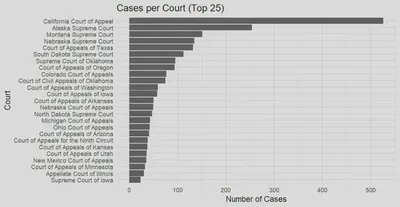
Volume by Court
# Top 25 jurisdictions
cases_df %>%
  count(court, sort = TRUE) %>%
  head(25) %>%
  ggplot(aes(x = reorder(court, n), y = n)) +
  geom_col(fill = "#bb0000") +
  coord_flip() +
  labs(
    title = "Top 25 Jurisdictions for ICWA Cases",
    x = "Court",
    y = "Number of Cases"
  ) +
  theme_minimal()
Next Steps
After downloading all data, including caselaw text and metadata, you can:
- Use Natural Language Processing to examine sentiment or common words
- Perform topic modeling to explore latent themes in ICWA cases
- Map filings by jurisdiction
- Integrate the data with other sources (e.g., demographic data, child welfare statistics)
Code Repository
The whole workflow is available on our GitHub repository.
Happy Coding!
Related Resources

Dr. Gia Elise Barboza-Salerno
Director
I am an interdisciplinary scholar whose research integrates law, public health, social work, and advanced statistics to study childhood adversity, violence-related harm, and neighborhood-level inequities. I lead the ISSUES Lab at Ohio State, translating spatial and legal analysis into policy and practice.